Introduction of Optical Flow Algorithm

1. Introduction
2. Assumptions
3. Formula Deducing
4. Attention
5. Reference and Further reading

Introduction

Optical Flow is a motion of a certain target in consecutive frames, which is caused by the motion of target, scene or camera. It reflects the image changes caused by motion in a small time interval to determine the direction and speed of motion of the image points.

Assumptions

Optical Flow provide the clue of motion recovering. It mainly depends on three assumptions:

1. [Constant light] The pixel light of target is constant in consecutive frames;
2. [Time sequence] The time interval of consecutive frames is so small that the change of time can be ignore when considering the motion change(This assumption is to be used for deducing the core formula of Optical Flow Algorithm);
3. [Neighborhood consistency] Neighbor pixels have the similar motion.

Formula Deducing

Assumed that the light of a certain pixel is in moment . After , this pixel has the same light with that in after a motion , means that.

$$I(x,y,t)=I(x+\Delta x,y+\Delta y,t+\Delta t)$$

Performing a first order taylor expansion on the right side of the equation, we can obtain a formula below.

$$I(x+\Delta x, y+\Delta y, t+\Delta t) = I(x,y,t) + I'_x\Delta x + I'_y\Delta y + I'_t\Delta t$$

means that.

$$I(x,y,t) = I(x,y,t) + I'_x\Delta x + I'_y\Delta y + I'_t\Delta t$$

therefore.

$$I'_x\Delta x + I'_y\Delta y + I'_t\Delta t = 0$$

It’s matrix format is like this;

$$\begin{bmatrix}I'_x & I'_y\end{bmatrix} \begin{bmatrix}\Delta x \\ \Delta y\end{bmatrix}=-I'_t \Delta t$$

where are partial derivative of light of in direction and , namely gradient. is the partial derivative of light of in moment . is the light difference of between consecutive frames. So , the equation can be written as that.

$$\begin{bmatrix}I'_x & I'_y\end{bmatrix} \begin{bmatrix}\Delta x \\ \Delta y\end{bmatrix}=-\Delta I_t$$

In consecutive frames, are known, are optical flow unknown.

According to assumption 3, the neighbor pixels have the same optical flow, we can choose a neighbor region centered on .

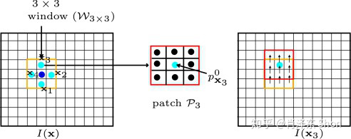
Considering all pixels in neighbor region, we can obtain a matrix formula.

$$\begin{bmatrix} I'^{(1)}_x,I'^{(1)}_y \\ I'^{(2)}_x,I'^{(2)}_y \\ \cdots \\ I'^{(n)}_x,I'^{(n)}_y \\ \end{bmatrix} \begin{bmatrix}\Delta x \\ \Delta y\end{bmatrix} = \begin{bmatrix} -\Delta I^{(1)}_t \\ -\Delta I^{(2)}_t \\ \cdots \\ -\Delta I^{(n)}_t \end{bmatrix}$$

The equation can be written as . Therefore, the solution of optical flow in can be compute by least square:

$$A^TAX=A^TB$$ $$X=(A^TA)^{-1}A^TB$$

Attention

The is required to be invertible. If not, it may cause a aperture problem. As the GIF shown left, the motion of stripe can not be detect through the circle aperture. So, Lucas and Kanade proposed selecting those “invertible” pixels for computing optical flow. This kind of pixels are usually some corner points, which are detected by Harris or other Algorithm.

Except mentioned above, Lucas and Kanade proposed using pyramid images to solve the problem caused by large offset. Eventually, Lucas-Kanade’s method was used to obtain sparse optical flow. The Lucas-Kanade method is a classical optical flow algorithm. Farneback proposed a method to obtain dense optical flow in 2003. The GIF below is the compare of sparse and dense optical flow.

In ICCV2015, a group proposed a deep learning method FlowNet to solve problems of optical flow estimation using CNN. In CVPR2017, the same group proposed a modified FlowNet2.0. FlowNet2.0 is the most popular paper in optical flow field since 2015.

Reference and Further reading

Farneback: https://blog.csdn.net/xholes/article/details/79894340

Flow Net: https://zhuanlan.zhihu.com/p/37736910

Flow Net: https://zhuanlan.zhihu.com/p/74460341